
[Back]

[Index]

[Next]
AIR FORCE PAMPHLET 14- 210 Intelligence
1 FEBRUARY 1998
 [Back] |
 [Index] |
 [Next] | USAF INTELLIGENCE TARGETING GUIDE AIR FORCE PAMPHLET 14- 210 Intelligence 1 FEBRUARY 1998 |
153
A5.2. Types of Ranking. A5.2.1. Ordinal Scale. One of the easiest methods of ranking target value involves the use of ordinal scales to assign factors a priority according to their relative worth. Target A may be more important or valuable than Target B but less valuable than Target C. It would be logical to infer that Target C is also more valuable than Target B. However, their absolute relationship remains unknown under this approach. Using this method, we may know that Target A is more important than Target B, but we do not know how much more important.
A5.2.2. Metric Scales. A second method of ranking targets would be to use metric or cardinal scales to determine their worth in some "real" sense. In a simple case, we can rank people by their ages. Joe might be 25 years old and Sam 37 years old. We can rank these individuals not only relatively but also absolutely. Relatively, Sam is older than Joe; absolutely, Sam is 12 years older than Joe. Thus, metric scales can apply to targets. For example, one airfield's runway is 2,000 feet longer than another's; one airfield has 25 more assigned aircraft than another. This method of ranking is most desirable but the most difficult, because there is rarely any single measure of their comparative value. A combination of measurements must be used. Usually the ways these factors are measured does not directly reveal their threat to friendly forces or value to the enemy.
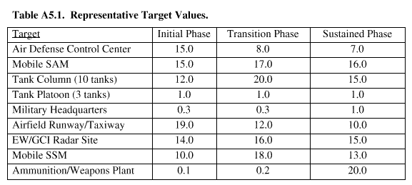
A5.2.3. Ratios. Another method is to develop a ratio of relative worth by determining, for example, that Target D is twice as important as Target E, and four times as important as Target F. However, this method does not measure each individual target's absolute value. Often a value of 1 is assigned to some baseline target, and all other targets are assigned values with respect to the baseline. The USAF Nonnuclear Consumables Annual Analysis (NCAA) uses this type of ranking, which recognizes that the relative value of targets can change over time during a conflict. This methodology divides the period of action into three phases: the initial or intense phase, covering the first 10 days of action; the transition phase, covering the next 20 days; and the sustained, or steady state phase, covering the remainder of the conflict. Target values for this type of ranking are determined by combining the independent assessments of several analysts. The final target value set is the weighted geometric mean of the values submitted. The baseline target in this methodology is a tank platoon, which is assigned an arbitrary value of one. Values for other targets are computed to determine their relative importance compared to the tank platoon, for the initial, transition, and sustained phases of the con-flict. Some representative target values for the three phases are shown inTableA5.1.. 153
A5.2.5. Aggregation Ranking. Targets can also be ranked by an aggregation of their specific char-acteristics. Does an airfield have an active air order of battle? What level of activity is apparent? Has the enemy sought to repair damage inflicted on the target? How concentrated have his efforts been? Is the target heavily defended? Are some of its elements hardened to protect them against attack? The answer to each of these questions is relative to the issue of relative target worth. Taken together, these factors can reveal important information that can lead to target ranking. Several statistical techniques may be used to combine these factors into measures of relative utility. The combination of measure-ment methods will be treated in the remainder of this section.
A5.3. Qualitative Analysis. Because the decision making process is constrained by time, costs, previous experiences, and perceptions of the participants, much decision making in the target development arena is based on qualitative rather than quantitative analysis. Since analysis occurs in an environment where power relationships, personal desires, and the necessity for coordination exist, problems can almost never be approached on a completely systematic basis. Many decisions are somewhat arbitrary, in that critical choices have already been made in selecting the alternatives. Much of targeting is concerned with value choices that can be explicitly described in words but are extremely difficult to express in the languages of mathematics or the computer.
A5.3.1. However, qualitative analysis is not a substitute for quantitative analysis. Both are useful and complementary techniques for structuring a problem to reach a rational conclusion. Both may be used to reduce uncertainty in decision making. Each technique has strengths that tend to diminish the lim-itations of the other.
A5.3.2. In targeting, qualitative analysis is the examination of potential targets to determine impor-tance, significance, and priority of attack based upon value choices which are not quantifiable. Qual-itative analysis is often necessary when precise information on quantities is unavailable. For example, the quantities of supplies reaching the enemy forces at the forward area has shown historic signifi-cance in the outcome of battles. Unfortunately, this effect is extremely difficult to quantify.
154
155
A5. 4.1. Since targeting decisions vary in complexity, quantitative analysis can be used in various ways. The numbers of people and organizational units affected, the degree of structural change required, and the costs of such changes are factors that determine the scope of a given decision situa-tion.
A5.4.2. The targeting decision maker has many quantitative models to choose from. These models tend to be either macrosystems or microsystems. Macrosystem analysis approaches a problem from an extensive point of view. It attempts to consider all of the variables that could contribute to, or extract value from, the proposed alternatives. For example, it might weigh the technical, political, economic, social, and aesthetic considerations that would lead to success in a given battle. Mac-roanalysis tends to take place at the higher levels of the DoD hierarchy where decisions concern broad allocation of resources, planning for major campaigns, and overall review of ongoing operations. At these levels, decision makers are not necessarily interested in the implications and overall impact of the specific situation. Microsystems analysis, on the other hand, approaches a problem from an inten-sive point of view, concentrating on a single variable, such as the cost of destroying a particular target. This approach leaves the consideration of remaining variables such as how to win the battle to other efforts. At lower levels, applications lean toward a micro approach, where decisions are made to ensure specific tasks are carried out effectively and efficiently.
A5.4.2.1. The use of models and quantitative analysis techniques in targeting offers many advan-tages. They allow planners to handle problems that are both large and complicated, allowing con-sideration of only the most relevant factors. They provide a risk- free, low- cost environment to test tactics and strategy before implementation.. Alternative courses of action can be recommended to the commander accompanied by impact analysis. Finally, the use of models makes it necessary to define the facts for a given problem and forces the decision making participants to state their feel-ings, objectives, values, and assumptions explicitly.
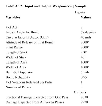
A5.4.3. Examples of Quantitative Analysis. A5.4.3.1. Simple Target Methodology . Most of these applications have been oriented toward examination of selected components of target systems. In the case of an aircraft delivery system, the weaponeering model attempts to grasp the physical characteristics of the aircraft as it moves through air space, the weapons as they strike the target and the resulting interaction of the weap-ons effects on the target structure. The weaponeering model of this problem considers a large number of details, ranging from the position of the aircraft in space to the geometry of the bombs hitting the ground. However, the model involves only one aircraft and one target. The situation and the scope of the models also limited by the assumption that the aircraft successfully reaches and acquires the target. TableA5.2.shows a sample set of inputs and outputs for a typical non- nuclear weaponeeringproblem. 155
A5.4.3.2.1. A typical approach using traditional weaponeering concepts would be to compute the probabilities of inflicting various types of damage on each of the components of the air-field separately. Thus, the runway would be weaponeered with a given number of aimpoints, while the hangarettes might be considered separately, as a single area (or set of area targets), and POL, storage areas, and support buildings would each be weaponeered separately.
A5.4.3.2.2. Another approach would be to treat the entire airfield as a single complex target. The separate components would be defined in the context of the larger model which considers all of the parts and their relationships to each other. A sample airfield with such geographic interrelationships is shown in figure A5.1.
156
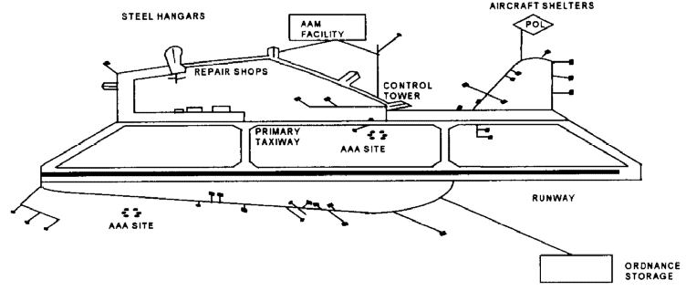
A5.4.3.2.3. After the airfield has been described, with appropriate structural descriptions and distance measurements, it is then possible to evaluate potential collateral damage on compo-nents near the selected target. For example, when the target is an aircraft shelter, the probabil-ity of cratering the taxiway would be evaluated. The problem of collateral damage can be computed with point or area targets, if either guided or unguided weapons are used. This com-plex model can be used to compute damage to targets offset from the aiming point and to determine damage probability for the target at the aiming point and any other target in close proximity. This approach makes it possible to evaluate all targets and their structural charac-teristics and sizes. The problem can also be solved using more complex methodologies based on simulation techniques.
A5.4.4. Target Utility Analysis. Target utility systems can be applied to problems of varying scope, ranging from large scale problems (strategic planning applied to an entire country) to small scale situ-ations. In this analysis technique, the utility or usefulness of different targets is weighed against the cost of attacking the target. Those targets with the highest pay- off at lowest losses are then prioritized. The following paragraphs is an example of how to use a subjectively derived weighing scheme to evaluate an attack against a complex installation such as an airfield.
A5.4. 4. 1. The concept of attacking enemy airfields is an integral part of counterair operations. However, its value depends largely on two factors: analysis of results to be achieved versus losses to be incurred, and the trade- off between the use of air assets for airfield attack as opposed to other missions.
A5.4.4.2. A number of factors must be considered in targeting airfields-- formidable air defenses; sheltering of aircraft; hardened command and support facilities; dispersed target elements at the main field and dispersal or forward operating bases which are equipped well enough to support air operations in the event the main operating bases are attacked. 157
158
A5. 4. 4. 4. Options could be arranged into categories. For example, in one case three general objectives could be of interest: the first would involve destroying aircraft; the second, cutting run-ways; and the third, destroying support areas. Under each of these options, TableA5.3.shows the following factors that must be considered:
Table A5.3. Example Options/ Factors Case.
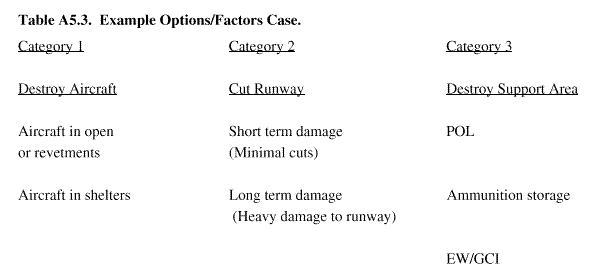
A5.4.4.5. The planner can assign these categories relative weights from a total pool of 100 points. For example, all 100 points could be assigned to Category 1 and none to categories 2 and 3 if the interest is only in destroying aircraft and not in closing the runway or destroying the support facil-ities. To emphasize each category, the 100 points could be distributed as follows: Category 1, 50 points; Category 2, 30 points; Category 3, 20 points. The decision maker must make the final decision as to the best combination of objectives.
A5.4.4.6. The second step is to assign weights within each category. For example, in Category 1 (Destroy Aircraft), the 100 points could be divided with aircraft in open or in revetments, 20 points, and aircraft in shelters, 80 points. This could be because all of the aircraft are equally important regardless of whether they are in the open, in revetments, or in shelters, but 80 percent of them may be in shelters in an attack.
A5.4.4.7. After all discussion and final agreement by the planners and other participants, the final assignment for all factors might be as shown in TableA5.4.:
158
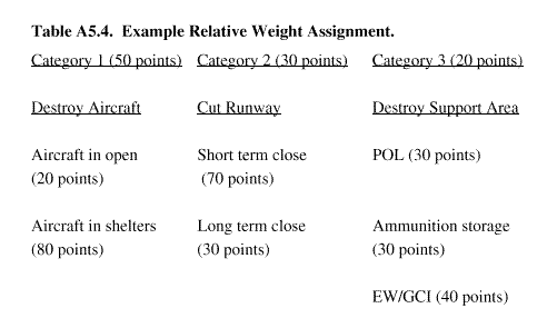
Figure A5.2. Fractional Bias Factor.
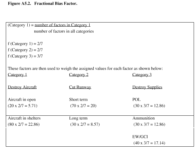
Fl = Aircraft in open = 5.71 x 50 = 285.5
F2 = Aircraft in shelters = 22.86 x 50 = 1143.0
F3 = Close Runway (Short term) = 20 x 30 = 600
F4 = Close Runway (Long term) = 8.57 x 30 = 257.1
F5 = Destroy POL = 12.86 x 20 = 257.2
F6 = Destroy Ammunition = 12.86 x 20 = 257 .2
F7 = Destroy EW/ GCI = 17.14 x 20 = 342.8
Finally, these weighted factors can be combined with probabilities of damage based on standard weap-oneering calculations into a single measure of effectiveness (EM) as follows:
EM = F 1 x Pd 1 + F 2 x Pd 2 + F 3 x Pd 3 + F 4 x Pd 4 + F 5 x Pd 5 + F 6 x Pd 6 + F 7 x Pd 7
A5.4.5. Expected Value Model. This example describes the use of a mathematical model developed around the concept of "expected value." Targets are defined in terms of size and relative worth. Weaponeering calculations provide estimates of potential levels of damage coverage or from a single sortie for each target. Targets and their associated factors are then combined into a scheme that lets us compare the impact of striking the target system one way versus another.
A5.4.5.1. In two target cases, for example, it is possible to compute the damage expected to each of the two targets over a range of application levels. Trade- offs can then be made between putting ordnance on one target or another. Keeping track of the total damage to be expected while making these tradeoffs allows us to find the optimum approach.
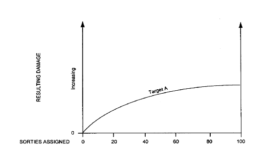
A5.4.5.2. It is possible to compute the expected damage from striking one target with one aircraft, a few aircraft, numerous aircraft, or with all the sorties that are available. The curve in figure A5.4 suggests the effects of striking a given target with varying numbers of sorties. The shape of the curve reveals that the more sorties allocated to damage the target, the harder it is to increase the
160
Figure A5.4. Sorties Allocated to the Illustrative Target. The shape of the curve reveals that the more sorties allocated to the target, the harder it gets to increase the damage level.
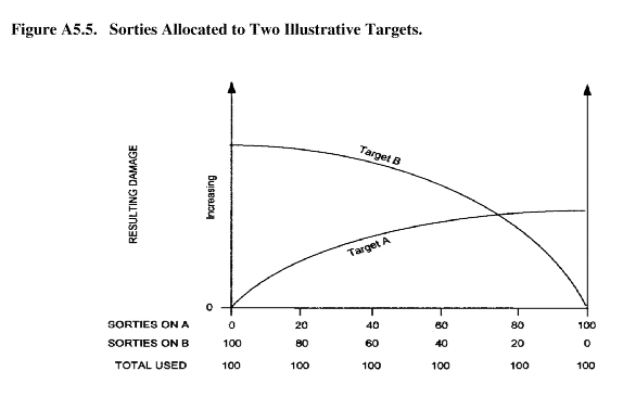
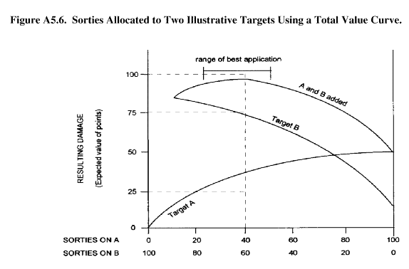
A5.4.5.3. Further defining the sample problem, assume that 100 aircraft sorties are available to allocate against two targets. They could all be assigned against the first target, all of them against the second target, or assigned between both targets. The diminishing return curves for both targets could be plotted on the same graph, constructing one from left to right and the other from right to left (figure A5.5). That is, if all sorties are allocated to Target A, then Target B will get none; if Target B gets all the sorties, then Target A will get none; and if Target A gets 20 sorties, then Tar-get B gets 80, and so forth. In its current state, the Y or vertical axis of the graph is dimensionless, representing relative levels of damage rather than absolute levels. 161
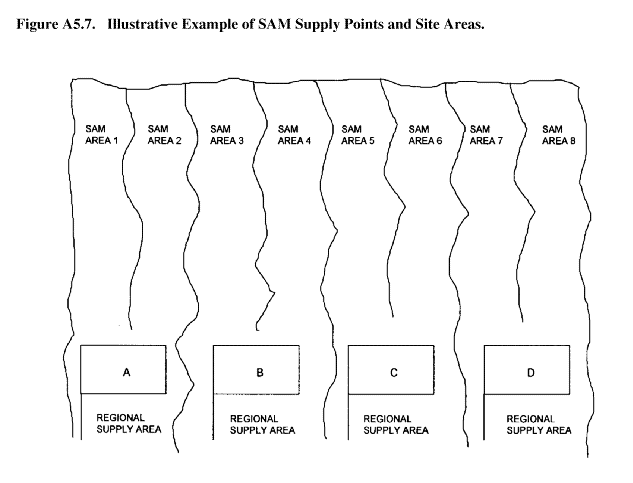
A5.4.6.1. There are four SAM supply points in a given area. Each supply point has a maximum of 50 missiles that can be used to resupply designated area sites. Each supply point has primary responsibility for two general SAM site areas. The sketch in figure A5.7 shows how these systems might be arranged. 163
164
165
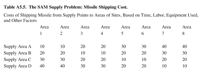
Table A5.6. The SAM Supply Problem: Possible Distribution of Missiles.
A5.4.6.4. When conducting operations against such a system, the commander is interested in the greatest possible disruption of resupply efforts. If enough attack forces were available, they might eliminate all four supply areas and all of the missile sites. However, when competition is high for the allocation of attack resources, it is not normally possible to perform such a devastating task. Therefore, a planner should examine the relative merits of destroying parts of the system. These merits can be measured in terms of equipment available to the enemy, costs associated with mov-ing the equipment around, or a combination of both approaches.
A5.4.6.5. As an example, if strikes eliminated the first supply area, the enemy would have to resupply from other, undamaged areas. Since the resupply capability of each area is limited, the most economical solution would be as shown in TableA5.7..Because it costs more to send mis-siles from supply area B to areas 1 and 2 than it didfromsupplyarea A, the total minimum cost of the effort to the enemy has been raised to 1000 cost units. Strikes that destroy both supply area A and supply area B make the enemy's resupply costs even higher, as shown in TableA5.8..
165


A5. 4. 6. 6. This sample application of the transportation problem to a targeting situation is rela-tively simple. Once the problem is appropriately structured, the relative merits of approaching the target system become more apparent. In the real world of targeting, problems are rarely this sim-ple. However, it is possible to use more elaborate models that include a greater level of detail, such as factors of resupply, exchanges between attacking aircraft and SAM sites, etc. Once the problem is appropriately structured, linear programming techniques already developed for the computer will determine relative solutions and give indications of their merits.
A5.4.7. Network Models in Targeting. The network model is also useful in targeting situations where it can be used to represent systems that have something flowing through them,( i. e., lines of communication, command networks, or power systems.) To illustrate this approach, an example based on a simplified representative power system is used. Figure A5.8 shows a power grid support-ing a city and the relationship among power sources, switching stations, and power lines. From this diagram, key points may be identified which, when destroyed, will have the greatest impact on the overall system.
166
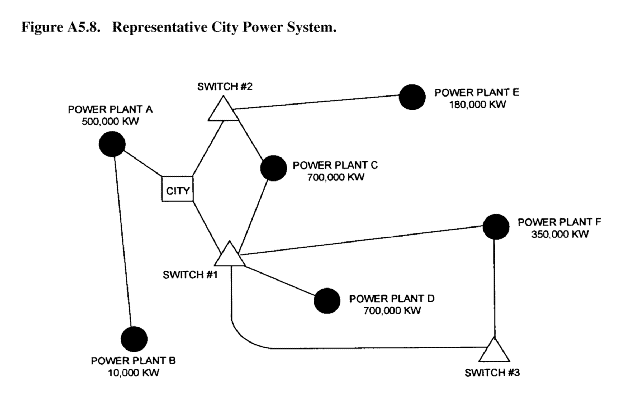
A5.4.7.2. Under normal conditions. it could be difficult to remove parts of a system. Weaponeer-ing techniques can compute the probabilities of success and the results would dictate the optimum allocation of available aircraft. All available sorties might be best used against Switch #1, or the sorties might be divided among the various power sources to produce the same effect. Although this example is greatly simplified, full network models can handle the hundreds of variables that comprise elaborate flow systems, and complex computer programs have been developed to handle such models.
A5.4.7.3. Lines of Communication (LOC) Network Mode . Several network models for LOCs are available for examining interdiction problems. Computer models have been developed to evaluate the capability of a transportation network to deliver supplies to destinations while road segments of the network are being successively destroyed and repaired. Initial models took an austere approach defining the logistical network in its simplest form. What roads are there? How are they connected? What is their capability to carry traffic? How many trucks are available? Similar models can be expanded to include additional costs (cost of repair, cost of interdiction, etc.) and other constraints (total repair capability, etc.). They can also account for the cushioning 167
Figure A5.9. LOC Network Example.
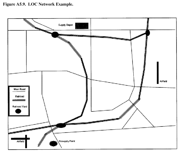
A5.4.7.3.1. One difficulty with an LOC network model is that it is a tremendous consumer of data. For example, thousands of road segments must sometimes be described to the computer and then constantly updated. The running of such models is expensive in terms of personnel, machines, and time.
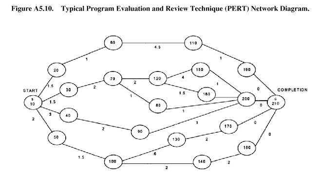
A5.4.7.4. Program Evaluation and Review Technique (PERT). Another useful tool is the spe-cialized version of PERT. PERT was originally developed in 1958 for use in managing the Polaris Fleet Ballistic Missile program. The missile program constituted the desired hardware, while PERT was a software development designed to aid in planning, scheduling, and controlling com-plex projects. Specific versions of PERT can be used to aid in the analysis of targeting problems. The first step in using it is to construct a network diagram of the problem so that the proper rela- 168
168 Page 169 170 169 tionship in the situation can be examined (figure A5.10). The PERT terms of reference for this network diagram include:
A5.4.7.4.1. Network. It is the pictorial description of the related series of events and activi-ties. All of these must be completed for the enemy to possess a particular capability. For example, producing aircraft requires the ability to manufacture the fuselage, engines, landing gear, and navigation and control systems.
A5.4.7.4.2. Event. An event is an identification of a requirement and does not represent any activity or time consumed. Thus, it can be either the initiation or completion of an activity, in a series of related activities. It is represented by a circle in the pictorial representation.
A5.4.7.4.3. Activity. Lines in the diagram represent the activities involved in moving from one event to another. The lines represent that time is being consumed in the cycle.
A5.4.7.4.4. Critical Path. The sequence of events is indicated by sequential numbering of each circle. The general direction of the arrows is from left to right. Time is expressed above each activity line in hours, days, and so forth. The longest path through the network of events and activities, in terms of time, is designated the critical path. Using PERT, one can determine what the critical path is and target it. This action can lengthen the enemy's time to complete the critical path and result in the delay or prevention of the enemy's completion of a product. Of note, targeting which increases the time of other paths may not delay the product unless it makes one of those paths greater than the critical path. Target analysis should also evaluate the vulnerability as well as the length of paths when determining the most efficient way to reduce enemy system output.
Figure A5.10. Typical Program Evaluation and Review Technique (PERT) Network Diagram.
A5.4. 8.1. The four- step decision tree technique is straight forward. First, identify the available options and the possible chance events that might occur. Second, draw the tree skeleton. Third, if probabilities are being expressed, enter the economic or statistical data and associated (subjective) probabilities. Finally, analyze the tree to determine the best course of action.
A5.4.8.2. The decision tree terms of reference include decisions, which are normally represented by squares; and change events, represented as circles. The connecting lines are termed branches and depict the alternate courses of action. The trees are normally drawn from left to right but may be drawn from top to bottom for easier presentation.
A5. 4. 8. 3. As an example, consider a patio party. There is a 40 percent chance of rain, and the party cannot be moved once the decision is made. There are only two options: inside or outside. The chance event is rain or no rain. Figure A5.11 illustrates the scenario.
Figure A5.11. Decision Tree.
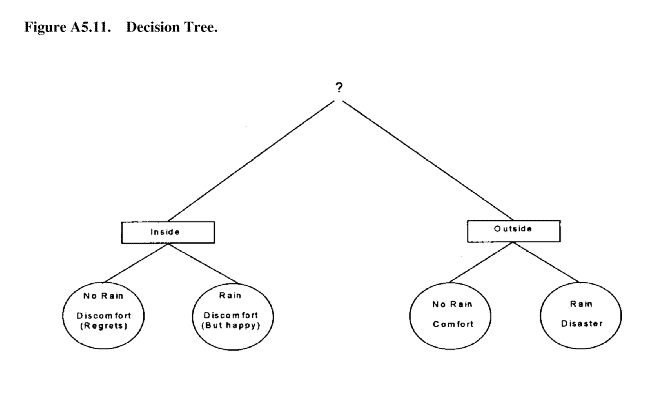
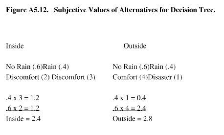
A5.4.8.4. Next, it is necessary to assess the subjective values of the alternatives in the circles. On an ascending scale, outside - no rain - comfort would rate "4" while outside - rain - disaster would be rate "1". Finally, it's 60 to 40 against rain. Figure A5.12 illustrates the results of multiplying the subjective value by the value of the chance event. Thus, there is a slight quantified edge (2.8 versus 2.4) for holding the party outside. The use of the decision tree gives the decision maker a 170
170 Page 171 172 171 simple graphic device, showing the areas where the analyst has been subjective and how that sub-jectivity affects the recommended course of action.
Figure A5.12. Subjective Values of Alternatives for Decision Tree.
A5.5. Substitutes for Quantitative Analysis. Because the decision making process can be constrained by time, costs, prior experiences, and perceptions, quantitative analysis is not always used. Since analysis occurs in an environment where power relationships, personal desires and the necessity for coordination exists, problems almost never can be approached exhaustively or on a completely systematic basis. Some alternatives to quantitative analysis follow.
A5.5.1. Intuition . There are two general approaches to this method of decision making. The first involves analytic reasoning by using logical models. Analytic reasoning reduces problems to a base of underlying causal relation. A logical model structured with an explicit set of axioms, premises, and assumptions is set forth, and all effort is directed toward detection of relationships. The decision vari-ables are manipulated in such a manner that some "optimal" equilibrium is reached to form the basis for a decision. The model produced is explicit and well defined, and its behavior can be deduced as logical consequences of its premises. Different people analyzing the same question should arrive at the same answer on the basis of logic alone.
A5.5.1.1. The second approach is a method of heuristic (trial and error) reasoning, using intuitive models and emphasizing workable solutions to total problem situations. The intuitive models may not have well- defined boundaries and are frequently not internally consistent. They are not derived from logic but are based on common sense, intuition, and unquantifiable feelings, making it difficult to determine the mechanisms at work. The heuristic analyst typically shifts thought patterns from one aspect of the situation to another, using loose definitions and bringing various parts of their knowledge to bear.
A5.5.2. Influence . Influence in the form of orders, advice, appeal to authority, or expertise, can come to the decision maker from several directions and can often replace analysis in decision making. An analyst may receive direction from a higher echelon or lateral pressure from personnel at equal levels which will significantly affect the decision. Also, subordinates often make suggestions, recom-mendations, and comments that also influence the decision.
171
A5.5.4. Habit . Experience can become a habit through repetitive responses. Habit has been called the most general and pervasive of all techniques for making decisions. The collective memories of members of an organization are vast encyclopedias of factual knowledge, habitual skills, and operat-ing procedures. These habits are in part provided by the organization, and in part brought in by new personnel who learned them in educational institutions or on previous jobs. Habits become standard operating procedures when they are accepted and internalized in the organization through formal writ-ten, and recorded programs.
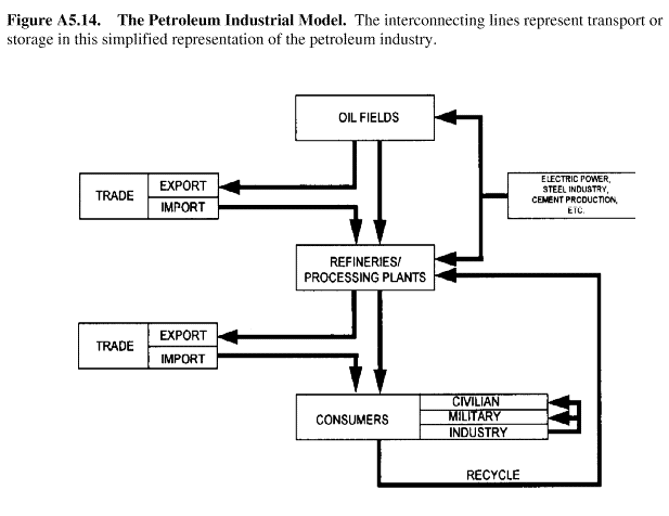
A5.6. "Target System Flow Charting" Analysis. In identifying target system components, specifying the activities of each component, and preparing an analysis model (steps two and three of target develop-ment), flow charting is a useful technique. An elaborate computer- based model is not always needed. A simplified model is often adequate. For example, the simplified basic industrial model shown here (figure A5. 13.) shows how the basic industrial model may be applied to a nation's petroleum industry (figure A5.14.).
Figure A5.13. Figure A5.13. The Basic Industrial Model.
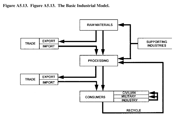
A5.6.1. The generalized component of the petroleum industry models are identified by the Functional Classification Coding System which identified nine broad groups of targets and their subgroups. Spe- 172
Figure A5.14. The Petroleum Industrial Model. The interconnecting lines represent transport or storage in this simplified representation of the petroleum industry.
A5.7. Critical Time Analysis. Critical time parameters are time- sensitive tasks that an enemy must complete effectively and efficiently to achieve its objectives. This analytical method is used to identify those time parameters and the task objectives, and to support target selection. For example, analysis might show that the critical time for an infantry unit is the 18- hour period immediately prior to launching an attack. The enemy's command and control system during that time may include vulnerable communi-cations links between commanders and their units. These communications channels contain directives and information that must be processed in the critical time. The pattern of signals could also indicate a unit's state of readiness for an attack. By targeting these communications channels for destruction or dis-ruption during the critical time, command and control could be degraded, thereby reducing the enemy's effectiveness. 173
 [Back] |
 [Index] |
 [Next] | USAF INTELLIGENCE TARGETING GUIDE AIR FORCE PAMPHLET 14- 210 Intelligence 1 FEBRUARY 1998 |